Forecast inventory demand 30 days out — by SKU, by region

The Problem

Inventory is the unsexy P&L lever that quietly destroys margin in fast-moving consumer businesses. Stockouts kill conversion at exactly the moment a customer is willing to spend. Over-ordering ties up working capital and forces end-of-season discounting that compresses margin for months.

The tooling most teams use looks something like this: one analyst, one Google Sheet of last year's sales by SKU, a column for "judgement adjustment", and a Friday meeting where the merchandising team argues. It works for the top 10% of SKUs that everyone has opinions about. It fails badly for the long tail of 4,000 SKUs where nobody has time to look.

Three structural problems make this worse:

• External signal blindness. Weather, competitor pricing, and promo cadence all move demand by 10-40%, and none of them are in the spreadsheet.
• Lead-time math is hard. Suppliers in different regions have lead times from 3 days to 9 weeks. A "30 day forecast" is meaningless without the lead-time overlay.
• The forecast is never re-run. The Monday spreadsheet ages to lies by Friday, but nobody wants to redo it.

⚠ Numbers below are illustrative. Real client data is confidential.

The DataCraves Approach

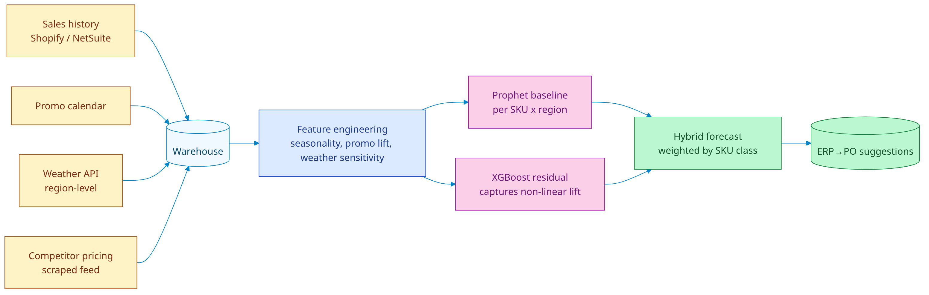
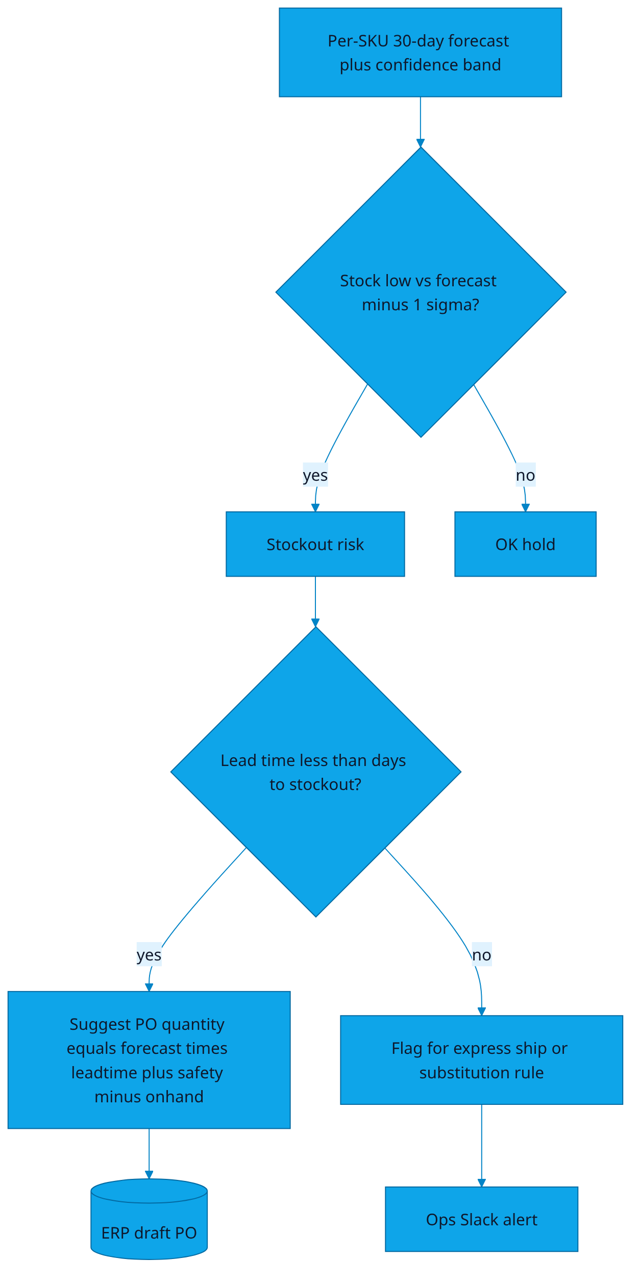
The Forecast Agent ingests sales history, the promo calendar, weather forecasts, and competitor pricing feeds. It produces a per-SKU × per-region 30-day demand forecast every night, with a 90% confidence band, and pushes PO suggestions to the ERP for any SKU heading for stockout inside its lead-time window.

We use a hybrid model — Prophet for the seasonal/trend baseline, an XGBoost residual model that captures non-linear lift from promos and weather. The two are blended per SKU class, weighted by which performed better on the trailing 60-day holdout.

Why hybrid, not pure ML

Pure XGBoost forecasts overfit on long-tail SKUs with sparse data. Pure Prophet misses the discontinuities caused by promos. Hybrid gives you the seasonality of one and the lift-modeling of the other, and lets you fall back to baseline when the residual model is uncertain.

The Math / The Logic

For each SKU × region pair, we compute three forecasts and blend:

# forecast_blend.py
from prophet import Prophet
import xgboost as xgb

def forecast_sku(history_df, exog_df, horizon=30):
    # 1. Prophet baseline — seasonality + trend
    p = Prophet(yearly_seasonality=True, weekly_seasonality=True,
                changepoint_prior_scale=0.05)
    p.fit(history_df.rename(columns={"date":"ds", "qty":"y"}))
    base_fc = p.predict(p.make_future_dataframe(periods=horizon))

    # 2. XGBoost residual — captures promo + weather lift
    resid_train = history_df["qty"] - base_fc["yhat"][:len(history_df)]
    feats = exog_df[["is_promo", "discount_pct", "temp_c",
                    "is_weekend", "competitor_price_idx"]]
    bst = xgb.XGBRegressor(n_estimators=300, max_depth=5,
                           learning_rate=0.05, subsample=0.85)
    bst.fit(feats[:len(history_df)], resid_train)
    resid_fc = bst.predict(feats[len(history_df):])

    # 3. Blend; weight by trailing-60d hold-out MAPE
    w_base, w_resid = blend_weights(base_fc, resid_fc, history_df)
    final = w_base * base_fc["yhat"][-horizon:] + w_resid * resid_fc

    return final, confidence_band(final, sigma=residual_std(history_df))

Reorder rule. For each SKU we maintain a target service level (default 95%, configurable per category). Reorder point is computed as:

reorder_point = forecast_lead_time + Z(0.95) * sigma_lead_time
suggest_qty   = forecast_(lead+review) + safety_stock - on_hand - on_order

Where Z(0.95) = 1.645 and sigma_lead_time is computed from the last 90 days of demand variance scaled to the lead-time window.

Sample Output / Insight

ROI Math

• Baseline. ₹50 Cr annual revenue, 12% margin, 4,000 SKUs, average inventory ₹8 Cr at any time, 6.2 inventory turns / yr, ~3% lost revenue from stockouts.
• Stockout reduction. 27% reduction → recovers ~0.8% of revenue ≈ ₹40 L / yr.
• Working-capital release. Better turns (6.2 → 7.4) → average inventory drops to ~₹6.7 Cr, freeing ₹1.3 Cr of working capital.
• Markdown reduction. Better matched supply → ~30% fewer end-of-season clearance markdowns ≈ ₹25 L margin saved.
• Total annualised value. ~₹1.95 Cr / yr in cash + margin. DataCraves Pro at ₹4,999/mo (~₹60K / yr) → 325× return.

Assumptions to challenge: figures assume promo cadence and weather signal are actually available. If you don't pipe weather, expect MAPE 3–4 pp higher and ROI ~30% lower.

Common Pitfalls